The Poisson distribution is modelling the number of events within a defined time interval or area. For example, counting variables such as the recruitment for a clinical study, the number of adverse events or the number of children in a family. Events must occur independent of the time since the last event, and with a known constant probability. In case two groups should be compared, the success probability should be similar in both groups. The Poisson distribution is a univariate discrete distribution. Since the expected value and the variance are identical, only one parameter is necessary to know the distribution.

The primary example of the use of the Poisson distribution in clinical trials is to model the recruitment of patients in the planning phase of a study. When designing the study, it can be of importance to predict the recruitment time and efficiency. As this can have consequences for example on the drug supply to the different study sites to meet the patient demands. Or, in case an interim analysis is planned it can have an impact on the power of the statistical test.

Poisson regressions allow for dependent variables to be censored at zero, and allow for non-continuous dependent variables, but the variance must be equal to the mean. If the variance is higher than the mean, the Poisson distribution has a lower variance than the actual data and is therefore not reflecting it accurately.

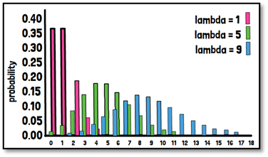
For the graphical presentation of the Poisson probability distribution function only bar graphs are valid since the distribution is discrete. Joining the values to a complete function is not applicable in discrete definition areas. Probability distributions help you decide the probability of a future event.

Here we can see three examples of probability distributions for different lambda, where lambda can be directly interpreted as the number of events that are expected for example in a certain time frame.